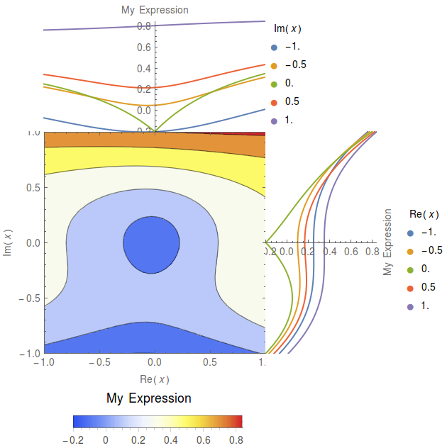
Visualizing functions that depend on a complex variable is oftentimes done with either contour plots or with multiple one dimensional plots where either the real or imaginary part is set to a selection of fixed values. This Mathematica function will combine both plots to provide the nice overview of the contour plot, while making it easy to compare it with the 1D lines.
An example:
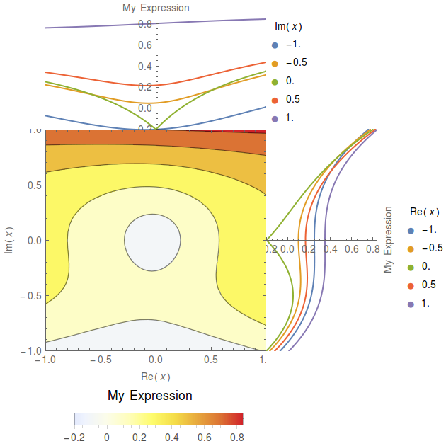
The option centerColormap can be used to assign the color in the “middle” of the color map (in this case white) to a fixed value,
which comes in handy, when e.g. zero has a special meaning and it is important whether we are below or above it. Applied to the last
example, this gives:
The code:
Above plots were created with
superComplexContourPlot[-1/3+(Abs[x]+1/10 Re[x]+Im[x]^3)/(1+Abs[x]),x,"My Expression"]
Respectively
superComplexContourPlot[-1/3+(Abs[x]+1/10 Re[x]+Im[x]^3)/(1+Abs[x]),x,"My Expression",centerColormap->True,centerColormapAt->0]
(where centerColormapAt->0 can be left out). To see the options of the command, type ?superComplexContourPlot. All other options
given to the function will be passed on to ContourPlot.